
The Physics department at USA develops students into scientists. The USA Physics faculty takes pride in knowing their students and preparing them for success in their academic endeavors. Undergraduate physics majors are given the opportunity and are encouraged to conduct research early in their undergraduate careers. The smaller size of the USA Physics Department creates a natural environment for students to interact with the department’s highly accomplished physics faculty members and generates opportunities for students to gain experience in the field in their undergraduate academic adventures. The Physics Department at USA welcomes you to take part in this experience!
What Can I do with a Degree in Physics?
Physics offers challenging, exciting, and productive careers. As a career, physics covers many specialized fields -- from acoustics, astronomy, and astrophysics to medical physics, geophysics, and vacuum sciences.
Physics offers a variety of work activities-lab supervisor, researcher, technician, teacher, manager. Physics opens doors to employment opportunities throughout the world in government, industry, schools, and private organizations.
Field of graduate study for physics bachelors in the U.S. one year after degree.

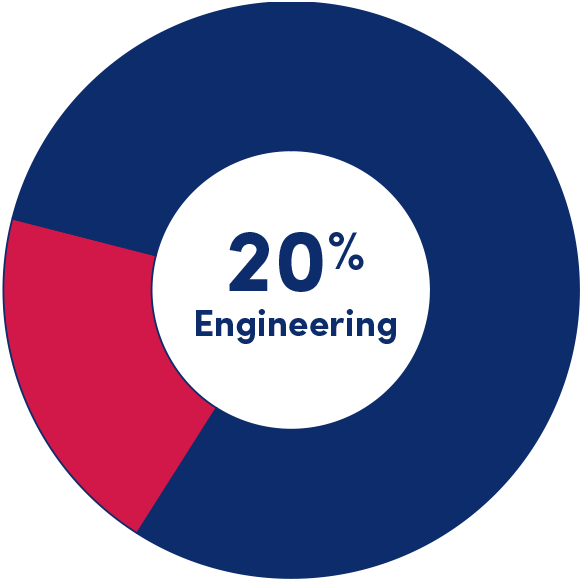

*Mathematics, Medicine, Education, Physical Sciences,
Computer Science, Social Science, Law, Business, Humanities, Other